지난 글에서는 디지털 옵션의 가격을 Closed Form으로 구해봤습니다.
2022.08.31 - [금융공학] - 디지털 옵션 #2. 디지털 옵션 Closed form 및 그래프
디지털 옵션 #2. 디지털 옵션 Closed form 및 그래프
이번 글 2022.08.30 - [금융공학] - 디지털 옵션 #1. 디지털 옵션이란? 수학공식은? 디지털 옵션 #1. 디지털 옵션이란? 수학공식은? 이번 글부터 시작하여 몇 회에 걸쳐 다룰 파생상품은 바로 디지털 옵
sine-qua-none.tistory.com
이번 글에서는 디지털 옵션을 MonteCarlo Simulation(MC)으로 구해보겠습니다. 먼저 MC를 살짝 복습해 볼까요?
MonteCarlo Simulation
지난 글들에서, 우리는
○ 델타원 상품 : 2022.08.08 - [금융공학] - Black Scholes Equation의 풀이: 시뮬레이션
○ 콜옵션 : 2022.08.21 - [금융공학] - 옵션 #6. 옵션 프리미엄 구하기 실습: MonteCarlo Simulation
○ UOC : 2022.08.29 - [금융공학] - 배리어옵션 - UOC 옵션 #4 MonteCarlo Simulation
의 상품을 MC를 이용해 구해봤습니다.
그런데 델타원 상품, 콜옵션과 UOC의 결정적인 차이가 무엇이었나요? UOC는 주가가 배리어를 상회하는 그 순간에 옵션이 끝나게 되므로 하루하루, 좁게는 매분 매 초의 주가 움직임이 모두 영향을 미칩니다. 배리어를 치면 끝나야 하는 상품이기 때문이죠. 반면에 델타원이나 콜옵션 상품의 경우 중간 주가 패스는 어찌 됐든 간에, 만기 때의 종가가 무슨 값이냐에 따라 페이오프가 결정되죠.
디지털 옵션은 어떤가요? 중간 주가 패스에 영향을 받는 페이오프가 아닙니다. 만기 종가만 관찰을 해서 페이오프가 어떻게 산출되는지만 보면 됩니다. 따라서 주가생성 빈도는 만기 한번입니다.
만기 시점 종가 생성
2022.06.19 - [금융공학] - GBM 주가패스 만들기 #1: 만기시점 주가만
GBM 주가패스 만들기 #1: 만기시점 주가만
이 글은 2022.06.07 - [금융공학] - 주식의 수학적 모델 #3 : GBM모델 주식의 수학적 모델 #3 : GBM모델 이 글은 2022.05.27 - [금융공학] - 주식의 수학적 모델 #1 주식의 수학적 모델 #1 이 글은 2022.05.25 - [..
sine-qua-none.tistory.com
을 복습해 보면, GBM 모델하에서 만기 주가 ST는
ST=S0exp((r−q−12σ2)T+σ√Tz) , z∼N(0,1)
의 식으로 분포를 구할 수가 있습니다. 여기서 T는 디지털옵션의 만기, S0는 현재가, r,q,σ는 각각 무위험 이자율, 기초자산의 연속 배당률, 기초자산의 변동성입니다.
디지털 옵션의 만기 페이오프
행사가 K를 기초자산이 넘으면 c2 쿠폰을, 기초자산이 행사가를 넘지 못하면 c1을 지급하는 상품이므로 만기 페이오프는
f(ST)=c1I(ST<K)+c2I(ST≥K)
로 유식하게 표현 가능합니다.
MonteCarlo Simulation
2022.08.08 - [금융공학] - Black Scholes Equation의 풀이: 시뮬레이션에서 다룬 내용에 따라
e−rTE(f(ST))≈=e−rT1NN∑i=1f(Si)
로 구할 수 있습니다. 여기서 N은 시뮬레이션 횟수이고 Si는 식(1)으로 생성한 만기 종가들이죠.
MonteCarlo Simulation의 Python Code
import numpy as np
import matplotlib.pyplot as plt
from scipy.stats import norm
import time

N = norm.cdf

def DigitalOption_MC(s0, strike, upCoupon, downCoupon, maturity, rfr, vol, div):
    nSimulation = 50000
    drift = (rfr - div - 0.5 * vol ** 2) * maturity
    diffusion = vol * np.sqrt(maturity)
    df_mat = np.exp(-rfr * maturity)

    payoff = []
    zNormal = np.random.normal(size=nSimulation)
    stock_mat = s0 * np.exp(drift + diffusion * zNormal)

    payoff = np.array([upCoupon if s >= strike else downCoupon for s in stock_mat])

    return payoff.mean() * df_mat

def DigitalOption_MC_process(s0, strike, upCoupon, downCoupon, maturity, rfr, vol, div):
    nSimulation = 100000
    drift = (rfr - div - 0.5 * vol ** 2) * maturity
    diffusion = vol * np.sqrt(maturity)
    df_mat = np.exp(-rfr * maturity)

    payoff = []
    zNormal = np.random.normal(size=nSimulation)
    stock_mat = s0 * np.exp(drift + diffusion * zNormal)

    payoff = np.array([upCoupon if s >= strike else downCoupon for s in stock_mat])
    cumulative_mean = np.cumsum(payoff)/np.arange(1,nSimulation+1) *np.exp(-rfr*maturity)
    exact_value = DigitalOption_ClosedForm(s0, strike, upCoupon, downCoupon, maturity, rfr, vol, div)

    plt.figure(figsize=(10, 10))
    plt.suptitle('digital option price by MC')
    sim_list = [100, 1000, 10000, 100000]

    for i in range(len(sim_list)):
        plt.subplot(2, 2, i + 1)
        plt.plot(cumulative_mean[:sim_list[i]], label='{} iteration'.format(sim_list[i]))
        plt.hlines(exact_value, 1, sim_list[i], color='r')
        plt.legend()

    plt.show()

def Calculate_DigitalOption():
    s0 = 100
    strike = 100
    upCoupon = 3
    downCoupon = 1
    maturity = 1
    rfr = 0.02
    vol = 0.2
    div = 0.01

    do_value_closedform = DigitalOption_ClosedForm(s0, strike, upCoupon, downCoupon, maturity, rfr, vol, div)
    do_value_mc = DigitalOption_MC(s0, strike, upCoupon, downCoupon, maturity, rfr, vol, div)

    print('Digital Option Value by ClosedForm : {:.3f}'.format(do_value_closedform))
    print('Digital Option Value by MC         : {:.3f}'.format(do_value_mc))

    DigitalOption_MC_process(s0, strike, upCoupon, downCoupon, maturity, rfr, vol, div)

def DigitalOption_ClosedForm(s0, strike, upCoupon, downCoupon, maturity, rfr, vol, div):
	# 생략

if __name__ == '__main__':
    Calculate_DigitalOption()
간략히 살펴보겠습니다.
def DigitalOption_MC(s0, strike, upCoupon, downCoupon, maturity, rfr, vol, div):
    nSimulation = 50000
    drift = (rfr - div - 0.5 * vol ** 2) * maturity	# GBM drift 항
    diffusion = vol * np.sqrt(maturity)		# GBM diffusion 항
    df_mat = np.exp(-rfr * maturity)	# 만기까지의 할인율

    payoff = []		# 만기 종가별 payoff를 담는 그릇
    zNormal = np.random.normal(size=nSimulation)	# 시뮬레이션 횟수만큼의 normal random 추출
    stock_mat = s0 * np.exp(drift + diffusion * zNormal)	# 시뮬레이션 횟수만큼의 만기종가 추출

    # 각각의 만기종가에 따른 digital option의 payoff를 구하여 페이오프 배열완성
    payoff = np.array([upCoupon if s >= strike else downCoupon for s in stock_mat])


    return payoff.mean() * df_mat	# payoff평균을 구하고 현재로 할인하여 리턴
# 이 함수는 시뮬레이션 횟수별 MC결과의 수렴성을 visualizing하기 위해 작성

def DigitalOption_MC_process(s0, strike, upCoupon, downCoupon, maturity, rfr, vol, div):
    nSimulation = 100000
    drift = (rfr - div - 0.5 * vol ** 2) * maturity
    diffusion = vol * np.sqrt(maturity)
    df_mat = np.exp(-rfr * maturity)

    payoff = []
    zNormal = np.random.normal(size=nSimulation)
    stock_mat = s0 * np.exp(drift + diffusion * zNormal)

    payoff = np.array([upCoupon if s >= strike else downCoupon for s in stock_mat])

	# 시뮬레이션 횟수까지 payoff 배열의 누적합 배열을 array(1,2,..,nSimulation) 배열로 나누어
    # cumulative mean 배열을 완성하고
    # 할인율(scalar형태)를 곱해 시뮬레이션 1,2,..,nSmulation 별 MC 결과를 구함
	cumulative_mean = np.cumsum(payoff)/np.arange(1,nSimulation+1) *np.exp(-rfr*maturity)
    exact_value = DigitalOption_ClosedForm(s0, strike, upCoupon, downCoupon, maturity, rfr, vol, div)

    plt.figure(figsize=(10, 10))
    plt.suptitle('digital option price by MC')
    sim_list = [100, 1000, 10000, 100000]	# 시뮬레이션 횟수가 백,천,만,십만일 때 결과를 보고싶음

    for i in range(len(sim_list)):
        plt.subplot(2, 2, i + 1)
        plt.plot(cumulative_mean[:sim_list[i]], label='{} iteration'.format(sim_list[i]))
        plt.hlines(exact_value, 1, sim_list[i], color='r')
        plt.legend()

    plt.show()
○ 유사한 코드를 2022.08.21 - [금융공학] - 옵션 #6. 옵션 프리미엄 구하기 실습: MonteCarlo Simulation글에서 다룬 적이 있으니 비교하여 보시기 바랍니다.
결과를 보도록 하겠습니다.
Digital Option Value by ClosedForm : 1.921
Digital Option Value by MC         : 1.928
전의 글에서 구했던 Closed Form 계산과 거의 유사합니다.
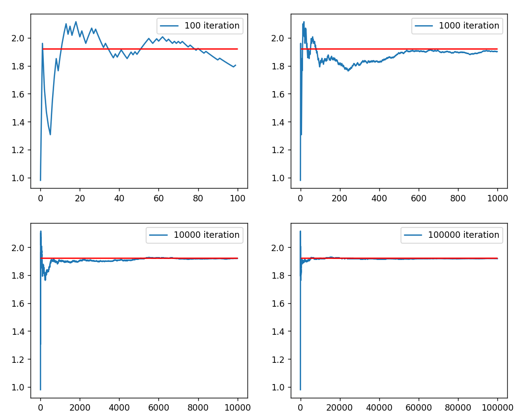
위 그림은 시뮬레이션 횟수별 MC 결과의 수렴 과정입니다. 처음 1,000회 정도까지는 요동치는 모습을 보이다가 샘플이 늘어날수록 안정적으로 수렴을 하죠.
이제, FDM 방법과 binomial tree로 계산하여 비교해 볼 일이 남았습니다. 다음 글에서 계속하겠습니다.
'금융공학' 카테고리의 다른 글
| 디지털 옵션 #5. 디지털 옵션 가격, Binomial Tree (0) | 2022.09.02 |
|---|---|
| 디지털 옵션 #4. 디지털 옵션 가격, FDM (0) | 2022.09.01 |
| 디지털 옵션 #2. 디지털 옵션 Closed form 및 그래프 (0) | 2022.08.31 |
| 디지털 옵션 #1. 디지털 옵션이란? 수학공식은? (0) | 2022.08.30 |
| 배리어옵션 - UOC 옵션 #5 Binomial Tree(이항트리) (0) | 2022.08.29 |


댓글